5. Enhancement by Histogram Manipulation

In the previous post on image types and formats, I used the histogram of a grayscale image to select the threshold for binary conversion. The histogram gives the distribution of pixels over various graytones or levels (PDF, Probability Distribution Function when normalized). Image enhancement can be done by manipulating the PDF of an image.

The original image with poor contrast and image enhanced by linear backprojection of the CDF

To increase the contrast of images, the pixels must be distributed over a wide range of gray levels. Histogram manipulation can be accomplished by using the CDF (Cumulative Distribution Function). The CDF is described by the following equation,

Definition of the Cumulative Distribution Function

A linear CDF would then do the trick of increasing PDF spread. Having CDF values plotted against itself would yield a linear plot. Each pixel must then take on its corresponding CDF value as its new gray level.

Notice that in the new PDF, pixels distribution are more spread especially at the 0-0.6 region. The old PDF is in 0-255 format since this is the default configuration of the imwrite() function. The new PDF is in 0-1.0 formats because it was taken from normalized values of the old CDF.

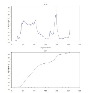
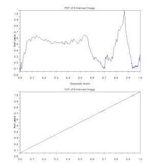
PDF and CDF of original image (left) and the enhance image (right)


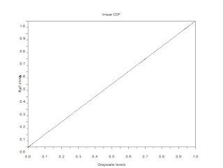
linear CDF as reference for backprojection

Aside from a linear CDF, a simple matrix manipulation can create a nonlinear CDF. A logarithmic CDF (y = log(x)) was applied. CDF values do not change in the white end of the scale and more pixels are concentrated in the dark region. Consequently, the result is a low contrast, dark image.

Image enhanced by a logarithmic CDF


PDF and CDF of image with logarithmic enhancement

Since I used histplot() on the last activity, I was fixated on how to access the values from histplot(). Histplot uses dsearch() which in turn makes use of tabul(). Thanks to the excellent Scilab Help modules. A simple use of find() by Gilbert Gubatan accomplishes the same thing. The difference with the latter is that tabul() does not store values for empty classes. In the case of the featured image, the length of the array is equal to 244 instead of 256. It is necessary to consider this in backprojection. Intuitively, one would index the CDF values with 0:255, which will not work for a 244 long array. See the code below.

Special thanks to Carmen Lumban who took the photo in 2008.

I give myself a 10/10 for this activity.

Code

A =imread('e_gray.jpg');
Amax = max(A);
Amin = min(A);

//get PDF of original image
p = tabul(A,'i');
scf(0); subplot(211);
plot(p(:,1),p(:,2)/max(p(:,2)));
title('PDF');
xlabel('Grayscale levels');
ylabel('# of pixels');

//get CDF of original image
c0 = cumsum(p(:,2)); //2nd col of p
c = c0/max(c0);
scf(0); subplot(212);
plot(p(:,1),c);
title('CDF')
xlabel('Grayscale levels');
ylabel('# of pixels');

//plot uniformly distributed CDF
x = c;
scf(1);
plot(x,x);
title('linear CDF');
xlabel('Grayscale levels');
ylabel('# of pixels');


//backplot uniform CDF to image

B = []; //enhanced image matrix
i = 0;
j = 0;
k= 0;

for i = 1:size(A,1)
for j = 1:size(A,2)
k = find(p(:,1)==A(i,j));
B(i,j) = c(k);
end
end

//get new PDF
p2 = tabul(B,'i');
scf(2); subplot(211);
plot(p2(:,1),p2(:,2)/max(p2(:,2)));
title('PDF of Enhanced Image');
xlabel('Grayscale levels');
ylabel('# of pixels');


//get new CDF
c02 = cumsum(p2(:,2)); //2nd col of p
c2 = c02/max(c02);
scf(2); subplot(212);
plot2d(p2(:,1),c2);
title('CDF of Enhanced Image');
xlabel('Grayscale levels');
ylabel('# of pixels');

C = []; //enhanced image, log
i = 0;
j = 0;
k= 0;
clog0 = abs(log(c));
clog = clog0/max(clog0);


for i = 1:size(A,1)
for j = 1:size(A,2)
k = find(p(:,1)==A(i,j));
C(i,j) = clog(k);
end
end

//get PDF of new image
p3 = tabul(C,'i');
scf(3); subplot(211);
plot(p3(:,1),p3(:,2)/max(p3(:,2)));
title('PDF of Enhanced Image: Logarithmic CDF');
xlabel('Grayscale levels');
ylabel('# of pixels');


//get new CDF
c03 = cumsum(p2(:,2)); //2nd col of p
c3 = c03/max(c03);
scf(3); subplot(212);
plot2d(p3(:,1),c3);
title('CDF of Enhanced Image: Logarithmc CDF');
xlabel('Grayscale levels');
ylabel('# of pixels');

imwrite(B, 'C:\Users\regaladys\Desktop\e_gray2.jpg');
imwrite(C, 'C:\Users\regaladys\Desktop\elog_gray2.jpg');