Lately I've been fascinated by these open-source graphics softwares - GIMP, Inkscape and Blender. GIMP is a raster graphics software similar to PhotoShop. Everyone in class is familiar with it when we used it an optics class last year. Inkscape on the other-hand is a vector graphics software. Best used with a tablet, Inkscape creations can be easily resized to whatever resolution (dpi) or dimension (pixel dimensions). Images are stored in Scalable Vector Graphics Format (.svg).
The prospect of coding my own filter and effects is something I look forward to as the lessons in this course progress. But before we proceed to the meaty codes ahead, here is a review of different image types and formats.According to the color or how color is mapped, digitized images can be categorized into 4 basic categories.
Binary Images, each pixel is either a black or a white and is represented by ones and zeros.
 Binary Image courtesy of NASA
 http://idlastro.gsfc.nasa.gov/idl_html_help/images/imgdisp01.gif
Size: 362x362
File Size: 5135
Format: GIF
Depth: 8
Storage Type: Indexed
Number of Colors: 256
Resolution Unit: centimeter
XResolution: 72
YResolution: 72
Grayscale images, each pixel has a value between white (255) and black (0). Color is limited to graytones. The following image is taken from NASA
Format: GIF
Depth: 8
Storage Type: Indexed
Number of Colors: 256
Resolution Unit: centimeter
XResolution: 72
YResolution: 72
Grayscale images, each pixel has a value between white (255) and black (0). Color is limited to graytones. The following image is taken from NASA
 Grayscale Image courtesy of NASA
 http://idlastro.gsfc.nasa.gov/idl_html_help/images/imgdisp02.gif
Size: 248x248
File Size: 10369
Format: GIFDepth: 8
Storage Type: Indexed
Number of Colors: 8
XResolution: 72.0
YResolution: 72.0
Truecolor images, the image is composed of channels in red, green and blue. The color of each pixel is determined by the superposition of each channel. The following jaguar fur is a sample of a trucolor image. Note on the image information that the number of colors is zero. Given that this is a truecolor image, it does not store an index of colors, hence the zero number of colors indicated.
 Truecolor Image of jaguar fur
courtesy of National Geographic
Size: 1280x1024
File Size: 357929
Format: JPEG
Depth: 8
Storage Type: Truecolor
Number of Colors: 0
XResolution: 100.0
YResolution: 100.0
File Size: 357929
Format: JPEG
Depth: 8
Storage Type: Truecolor
Number of Colors: 0
XResolution: 100.0
YResolution: 100.0
Indexed Images differ from truecolor in that color information is compressed into a single index of colors. This allows compression of an image to a smaller file size.
 indexed image
http://upload.wikimedia.org/wikipedia/en/7/7c/Adaptative_8bits_palette_sample_image.png indexed image
Size: 150x200
File Size: 25575
Format: PNG
Depth: 8
Storage Type: Indexed
Number of Colors: 256
XResolution: 72
YResolution: 72
Format: PNG
Depth: 8
Storage Type: Indexed
Number of Colors: 256
XResolution: 72
YResolution: 72
Advanced Image Types
With the expansion of imaging to fields like medicine and astronomy, advanced image types have surfaced. Here are some examples of advanced image types.
Multispectral images scan every pixel at different bands. For the Landsat, topographical images are taken up to 7 bands (3 for RGB and 4 for various IR bands). Information can be used for coastal area mapping, differentiating vegetation and snows from clouds among other meteorological applications. Hyperspectral images on the other hand take images from IR to visible and UV. One can imagine having the spectra of each pixel.
 Southeastern Indonesia
Taken by Landsat
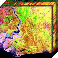 Hyperspectral cube, plane seen here is the visible spectra information, the sides of the cube are the edges of images taken in UV and IR bands. Photo taken by NASA
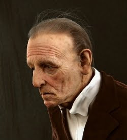 Image taken by setting up a virtual camera and lighting to take a picture of a 3D old man
Blender rendered by Kamil Mikawski
File Formats
Various image types differ on the kind of information stored recording images. These information can be stored or compressed in various file formats. Wikipedia gives a rundown of standard file formats. It surprised me that wiki documented 233 different file formats in existence. Formats like EMF (enhanced metafile) and SGB are supported only by Microsoft and Sun Microsystems respectively for their own software. There are also patented formats (HD Photo by Microsoft), and those created for Mars Rovers (ICER).
The most common image formats however, are TIF, BMP, GIF, PNG and JPEG.
BMP (bitmap) - 1 to 32-bit color depth/ supports transparencies and indexed color
GIF (Graphics Interchange Format) - 1 to 8-bit color depth/ support indexed color, transparencies, layers and animation/
JPEG (Joint Photographic Experts Group) - 8, 12, 24-bit color depth
PNG (Portable Network Graphics) - 1, 2, 4, 8, 16, 24, 32, 48, 64-bit color depth/ supports transparencies and indexed color
TIFF (Tagged Image File Format) - 1, 2, 4, 8, 16, 24, 32-bit color depth/ supports indexed color, transparencies and layers
Color depth refers to the representation of each pixel in bits.
Compression of these formats can either be lossy or lossless. In lossless, the original can be reconstructed from the compression. PNG and GIF use lossless compression while TIFF and JPEG can use lossy compression. This is also the same for other file formats.
With the expansion of imaging to fields like medicine and astronomy, advanced image types have surfaced. Here are some examples of advanced image types.
Multispectral images scan every pixel at different bands. For the Landsat, topographical images are taken up to 7 bands (3 for RGB and 4 for various IR bands). Information can be used for coastal area mapping, differentiating vegetation and snows from clouds among other meteorological applications. Hyperspectral images on the other hand take images from IR to visible and UV. One can imagine having the spectra of each pixel.
Southeastern IndonesiaTaken by Landsat
 Hyperspectral cube, plane seen here is the visible spectra information, the sides of the cube are the edges of images taken in UV and IR bands. Photo taken by NASA
 Image taken by setting up a virtual camera and lighting to take a picture of a 3D old man
 Blender rendered by Kamil Mikawski
File Formats
Various image types differ on the kind of information stored recording images. These information can be stored or compressed in various file formats. Wikipedia gives a rundown of standard file formats. It surprised me that wiki documented 233 different file formats in existence. Formats like EMF (enhanced metafile) and SGB are supported only by Microsoft and Sun Microsystems respectively for their own software. There are also patented formats (HD Photo by Microsoft), and those created for Mars Rovers (ICER).
The most common image formats however, are TIF, BMP, GIF, PNG and JPEG.
BMP (bitmap) - 1 to 32-bit color depth/ supports transparencies and indexed color
GIF (Graphics Interchange Format) - 1 to 8-bit color depth/ support indexed color, transparencies, layers and animation/
JPEG (Joint Photographic Experts Group) - 8, 12, 24-bit color depth
PNG (Portable Network Graphics) - 1, 2, 4, 8, 16, 24, 32, 48, 64-bit color depth/ supports transparencies and indexed color
TIFF (Tagged Image File Format) - 1, 2, 4, 8, 16, 24, 32-bit color depth/ supports indexed color, transparencies and layers
Color depth refers to the representation of each pixel in bits.
Compression of these formats can either be lossy or lossless. In lossless, the original can be reconstructed from the compression. PNG and GIF use lossless compression while TIFF and JPEG can use lossy compression. This is also the same for other file formats.
Grayscale images, treshold and conversion
RGB images are easily converted to grayscale with scilab's SIP toolbox functions im2gray and gray_imread.
Last week, I tried using Inkscape to practice making pixel art, an art form making it's comeback from the 80s. Here is a sample of three spaceship/hearts in different colors. Using the following code, the image was read and converted to grayscale,
Img = gray_imread('5.jpg');
histplot([0:0.05:1.0], Img)
imwrite(Img, 'C:\Users\regaladys\Desktop\5_gray.jpg');
histplot([0:0.05:1.0], Img)
imwrite(Img, 'C:\Users\regaladys\Desktop\5_gray.jpg');


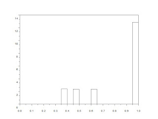
A histogram then displays the distribution of the pixels over different graylevels (Probability Distribution Function or PDF). Those at the 0 end are the darker pixels and a level of 1.0 means the pixel is white. Graylevel values are from 0 to 255 and is normalized by the histplot function.
 Graytones of the converted pixel art image
The histogram is useful in determining the threshold level for binary conversion. Values over the threshold level are converted to white and lower values are converted to black. Adjusting the treshold level can remove a lighter background or unwanted elements in the image.
The PDF information of the pixelships shows pixel concentrations at 1.0 and three other gray-levels. Binary conversion at different threshold values can remove one of the pixelships. Binary conversion of a grayscale is executed in a line of code.
Img=im2bw('5_gray.jpg', 0.8);
imwrite(Img, 'C:\Users\regaladys\Desktop\5_black1.jpg');

threshold at 0.8

threshold at 0.6

threshold at 0.45
Another example is Nat Geo's jaguar fur wallpaper. With a more diverse range of shades and hues, the PDF of this image is more spread. In binary conversion of the image, I wanted to isolate the jaguar's spots. This requires a threshold of around 0.25.


During conversion, image dimensions (matrix size) were not changed. But with lower amounts of color information, file sizes decrease after grayscale and binary conversion (312 KB for the truecolor image, 39.6 KB and 54.3 KB for the grayscale and binary conversions).
Binary conversion is also useful in cleaning up grayscale text scans. Here is Activity 1's plot taken from an old journal and the clean-up by binary conversion.
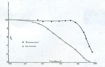
Scanned scientific plot from an old journal
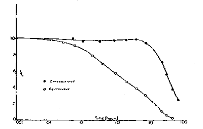
Binary version of the scanned plot removes the unwanted background color
For this activity I give myself a 9/10. Most of the difficulty in the activity was encountered during the image conversion. Also writing and editing take up more time than the actual research. This blog though is an exercise to write the next blog entries more efficiently. It was fun creating the entries but it can also become a form of distraction from coursework. Making these entries are so addicting. hehehe.
On the more technical side, one must remember to increase stacksize and use images with smaller dimensions.
I would like to thank wifi hotspots, Mushroomburger and McDonalds in Katipunan that housed me for several nights to complete the activities.
References
Scilab 4.1.2 Documentation
M. Soriano. A3 - Image Types and Formats. NIP, University of the Philippines. 2010.
Remote Sensing Tutorial. NASA. http://rst.gsfc.nasa.gov/
Geoscience Australia. http://www.ga.gov.au/
www.blender.org
www.wikipedia.com
The PDF information of the pixelships shows pixel concentrations at 1.0 and three other gray-levels. Binary conversion at different threshold values can remove one of the pixelships. Binary conversion of a grayscale is executed in a line of code.
Img=im2bw('5_gray.jpg', 0.8);
imwrite(Img, 'C:\Users\regaladys\Desktop\5_black1.jpg');

threshold at 0.8

threshold at 0.6

threshold at 0.45
Another example is Nat Geo's jaguar fur wallpaper. With a more diverse range of shades and hues, the PDF of this image is more spread. In binary conversion of the image, I wanted to isolate the jaguar's spots. This requires a threshold of around 0.25.


Jaguar fur in truecolor, grayscale and binary conversions using Scilab
During conversion, image dimensions (matrix size) were not changed. But with lower amounts of color information, file sizes decrease after grayscale and binary conversion (312 KB for the truecolor image, 39.6 KB and 54.3 KB for the grayscale and binary conversions).
Binary conversion is also useful in cleaning up grayscale text scans. Here is Activity 1's plot taken from an old journal and the clean-up by binary conversion.

Scanned scientific plot from an old journal

Binary version of the scanned plot removes the unwanted background color
On the more technical side, one must remember to increase stacksize and use images with smaller dimensions.
I would like to thank wifi hotspots, Mushroomburger and McDonalds in Katipunan that housed me for several nights to complete the activities.
References
Scilab 4.1.2 Documentation
M. Soriano. A3 - Image Types and Formats. NIP, University of the Philippines. 2010.
Remote Sensing Tutorial. NASA. http://rst.gsfc.nasa.gov/
Geoscience Australia. http://www.ga.gov.au/
www.blender.org
www.wikipedia.com
No comments:
Post a Comment