4. Area Estimation for Images with Defined Edges

With Green's Theorem one can easily calculate the area of images. This requires defined edges and Scilab with the SIP Toolbox accomplishes edge detection with follow().

Img = imread('circle.bmp');
[x,y] = follow(Img);
plot2d(x,y, rect = [0,0,200,200]);

l = length(x);
area = 0;
area_updated = 0;
for i=1:l-1
area_add = (x(i)*y(i+1)) - (x(i+1)* y(i));
area_updated = area_updated + area_add;
end

area = area_updated/2;

plot2d() displays the edges of the image defined in matrix [x,y]. Area is calculated in terms of pixels. The analytic value of the area is the number of pixels defining the image. With a white image, each matrix element is of the value 1. The area is simply given by sum(). Accuracy of the measurement is calculated by taking the difference of calculated area and the analytic value.

area_pixel= sum(Img);
dif = area - area_pixel;
area_acc = abs(dif*100/area_pixel);

Using synthetic images generated with Scilab, I calculated their areas with Green's Theorem.

Synthetic images with calculated areas of up to 97.8% and 97.3% accuracy

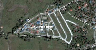
With the available satellite images of Wikimapia, I was able to take images of the subdivision where we live in Bacolod City.

Satellite image of St. Benilde Homes, Mansilingan City
It appears to be taken before 2006
photo courtesy of Wikimapia

Zooming in on Block 5, the Regalado Residence is indicated by the cross marking
photo courtesy of Wikimapia

I intend to calculate the total area of the subdivision and Block 5. To create solid bw images of these photos I used GIMP 2.6. I used the free select tool to create a mask of the block's shape and filled a white layer with black.

Black and white bitmap file of Block 5 for image detection and area estimation

With the map's scale, the conversion is approximately 5.25 m/pixel. This is calculated with the method described in Activity 1.

The area was calculated to 95.6% accuracy with the block measuring up to 11,103 square meters by area estimation and 11,620 square meters as the analytic value.

Here is the full code used to calculate the Block 5 area. Note that the bitmap file is a truecolor image though it appears to be in black and white. It must be first converted to a binary image before area estimation. Without this step, follow() function will not detect images as the truecolor file will have 3 channels for RGB, not compatible for the operation of follow().

//area estimation by green's function

Img = gray_imread('block5_w2.bmp');
histplot([0 : 0.05 : 1.0], Img)
Img2 = im2bw(Img, 0.5);

[x,y] = follow(Img2);
plot2d(x,y, rect = [0,0,200,200]);

l = length(x);
area = 0;
area_updated = 0;
for i=1:l-1
area_add = (x(i)*y(i+1)) - (x(i+1)* y(i));
area_updated = area_updated + area_add;
end

area = area_updated/2;
area_pixel= sum(Img);
dif = area - area_pixel;
area_acc = 100 - abs(dif*100/area_pixel);

Thanks to Ricardo Fabri, author of most of SIP, for keeping beautiful and simple docstrings on his macros. It took me a while to realize that the .bmp file must be converted to a binary image. Nevertheless, I have completed this exercise with more ease than the previous two. I feel a considerable improvement in my familiarity with Scilab and SIP.

For this activity I give myself a 10/10. I think this entry has achieved a simpler format in comparison to the previous discussions. Thanks to "Mother Earth" (mom) for reading this blog and telling me that she cannot understand anything. It has compelled me to write simpler and I hope to post more entries in the future.